Tidycensus and this Blog
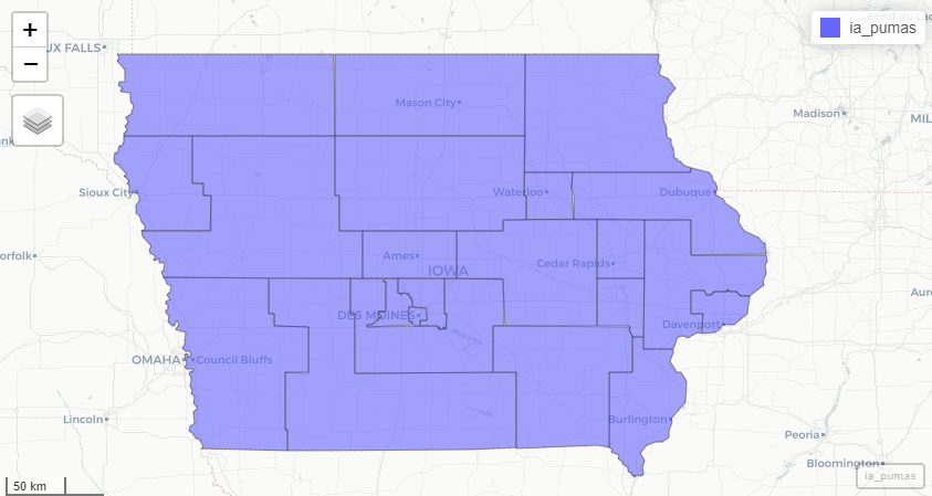
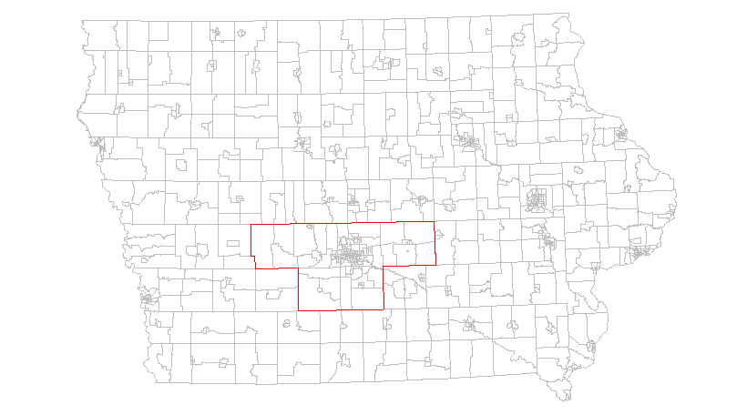
We watched videos learning about the basics of Tidycensus from the developer of the package. It taught basic map creation and general use of the application link to video I made one of the graphics from the video and one from his textbook online (I excluded the images made with the walk through). This blog was also created during the second week. Otherwise we started to look into our project.
library(tigris)
library(mapview)
options(tigris_use_cache = TRUE)
ia_pumas <- pumas(state = "IA", cb = TRUE, year = 2019)
ia_puma_map <- mapview(ia_pumas)
DM_IA_tracts <- map_dfr(c("IA"), ~{
  tracts(.x, cb = TRUE, year = 2021)
}) %>%
  st_transform(8528)

DM_metro <- core_based_statistical_areas(cb = TRUE, year = 2021) %>%
  filter(str_detect(NAME, "Des Moines")) %>%
  st_transform(8528)

ggplot() +
  geom_sf(data = DM_IA_tracts, fill = "white", color = "grey") +
  geom_sf(data = DM_metro, fill = NA, color = "red") +
  theme_void()
There are many more cool graphs to make with this library that I did not touch. Between Kyle Walker’s free book online and his lectures on YouTube there is tons to learn and do with the census data using this library. Hopefully this will be helpful later in our project and I will get to learn more.